![]()
Geometry / Involute
Authors: Chad Glinsky
Description: Mathematical review of the involute curve and its significance to mechanical gear systems.
Notebook imports and settings
%matplotlib inline
from helper import hide_toggle, round_degrees
from ipywidgets import interact, interactive
import matplotlib.pyplot as plt
from math import pi, hypot, ceil, cos
import numpy as np

# notebook modules
import involute as inv

# settings
FIGSIZE = (6, 6)  # size of plots
INTERACTIVITY = False  # static or interactive plots
# DEVELOPMENT USE: %autoreload 1
# PRODUCTION USE: %autoreload 0
%load_ext autoreload
%autoreload 0
%aimport involute
Introduction
An involute, specifically a circle involute, is a geometric curve that can be described by the trace of unwrapping a taut string which is tangent to a circle, known as the base circle.
Circle involute from an unwrapped string
Image credit: Wolfram MathWorldMathematics
The mathematics of a circle involute curve is reviewed here.
Nomenclature
| Symbol | Description |
|---|---|
| $r_b$ | Base radius |
| $\psi$ | Roll angle |
| $x$ | Cartesian x-coodinate |
| $y$ | Cartesian y-coordinate |
| $\kappa$ | Curvature |
| $R$ | Radius of curvature |
| $\alpha$ | Pressure angle |
| $\text{inv }\alpha$ | Involute function of pressure angle $\alpha$ |
Parametric Curve
An involute curve can be expressed by parametric equations in planar coordinates.
$$x = r_b (\cos\psi + \psi \sin\psi)$$$$y = r_b (\sin\psi - \psi \cos\psi)$$These equations specifically define an involute for a circle positioned at (0, 0) and the involute base starting at a polar angle of zero in the $xy$ plane
# interactive variable limits
r_base_lim = (1.0, 2.0)
roll_angle_lim = (0.0, 3.0)
r_max = ceil(hypot(*inv.involute_curve(max(r_base_lim), max(roll_angle_lim))))

# interactive callback function
def f(radius_base, roll_angle):
    fig = plt.figure(figsize=FIGSIZE)
    ax = fig.add_subplot(1, 1, 1)

    # base circle
    x, y = inv.circle_curve(radius_base, np.linspace(0, 2 * pi))
    ax.plot(x, y, '--')

    # involute curve
    roll_angles = np.linspace(0, roll_angle, num=100)
    x, y = inv.involute_curve(radius_base, roll_angles)
    ax.plot(x, y, '-', linewidth=2.5)

    # plot format
    ax.set_aspect('equal')
    plt.ylim(-r_max, r_max)
    plt.xlim(-r_max, r_max)
    plt.xlabel('x')
    plt.ylabel('y')
    plt.legend(['base circle', 'involute curve'])
    plt.grid()
    plt.show()

if INTERACTIVITY:
    print('Slider controls only work when running Jupyter.  They do not work in an HTML view.')
    interactive(f, radius_base=r_base_lim, roll_angle=roll_angle_lim)
else:
    f(r_base_lim[-1], roll_angle_lim[-1])

Curvature
The curvature, $\kappa$, of any point on a curve is defined as the reciprocal of the radius of curvature, $R$, at that point.
$$\kappa = \frac{1}{R}$$For a circle involute, the center of curvature and radius of curvature at any point is apparent based on its construction via an unwrapping string. Center of curvature always lies on the base circle, making the radius of curvature equal to roll distance.
# interactive variable limits
r_base_lim = (1.0, 2.0)
roll_angle_lim = (0.0, 3.0)
r_max = ceil(hypot(*inv.involute_curve(max(r_base_lim), max(roll_angle_lim))))

# interactive callback function
def f(radius_base, roll_angle):
    fig = plt.figure(figsize=FIGSIZE)
    ax = fig.add_subplot(1, 1, 1)

    # curvature at curve endpoint
    _, _, x_ctr_k, y_ctr_k = inv.involute_curvature(radius_base, roll_angle)

    # base circle
    phi_endpoint = np.arctan2(y_ctr_k, x_ctr_k)
    x, y = inv.circle_curve(radius_base, np.linspace(0, phi_endpoint))
    ax.plot(x, y, '--')

    # involute curve
    roll_angles = np.linspace(0, roll_angle, num=100)
    x, y = inv.involute_curve(radius_base, roll_angles)
    ax.plot(x, y, '-', linewidth=2.5)

    # plot - radius of curvature
    ax.plot([x_ctr_k, x[-1]], [y_ctr_k, y[-1]], '-')

    # plot - center of curvature
    ax.plot(x_ctr_k, y_ctr_k, 'kx')

    # remaining base circle
    x, y = inv.circle_curve(radius_base, np.linspace(phi_endpoint, 2 * pi))
    ax.plot(x, y, ':')

    # plot format
    ax.set_aspect('equal')
    plt.ylim(-r_max, r_max)
    plt.xlim(-r_max, r_max)
    plt.xlabel('x')
    plt.ylabel('y')
    plt.legend(['base circle', 'involute curve', 'radius of curvature', 'center of curvature'])
    plt.grid()
    plt.show()

if INTERACTIVITY:
    print('Slider controls only work when running Jupyter.  They do not work in an HTML view.')
    interactive(f, radius_base=r_base_lim, roll_angle=roll_angle_lim)
else:
    f(r_base_lim[-1], roll_angle_lim[-1])

Gearing
The involute is important to mechanical gears because it enables the transfer of mechanical power between rotating bodies without relying on friction as the mechanism of torque transfer, such as a car tire on a road surface. Furthermore, the rotational speed and torque can be modified during this transfer of power, enabling gear systems to change speed and torque between different points in the system.
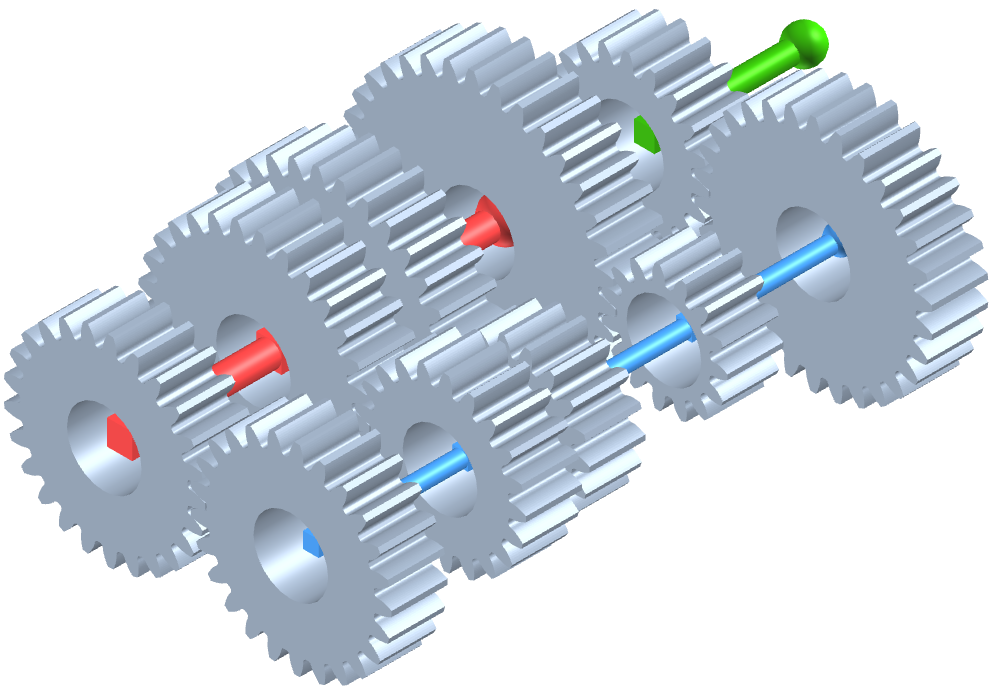
Involute gearing modeled in Gears App
Pressure Angle
The pressure angle for an arbitrary point on an involute curve is the angle between its radius vector and line tangent to the involute. As evident in the figure below, the involute base radius is related to the pressure angle at an arbiturary radius on the involute curve.
$$ r_b = r \cos\alpha $$
Involute curve diagram
Involute Function
The involute function is mathematically expressed as a function of pressure angle.
$$\text{inv }\alpha = \tan\alpha - \alpha$$The involute function can also be used to express the relationship between pressure angle and roll angle. The previous figure illustrates the involute function in the context of the roll angle and pressure angle.
$$\text{inv }\alpha = \psi - \alpha$$# interactive variable limits
r_base_lim = (1.0, 2.0)
roll_angle_lim = (0.0, 3.0)
r_max = ceil(hypot(*inv.involute_curve(max(r_base_lim), max(roll_angle_lim))))
# interactive callback function
def f(radius_base, roll_angle):
fig = plt.figure(figsize=FIGSIZE)
ax = fig.add_subplot(1, 1, 1)
# curvature at curve endpoint
_, _, x_ctr_k, y_ctr_k = inv.involute_curvature(radius_base, roll_angle)
# base circle
phi_endpoint = np.arctan2(y_ctr_k, x_ctr_k)
x, y = inv.circle_curve(radius_base, np.linspace(0, phi_endpoint))
ax.plot(x, y, '--')
# involute curve
roll_angles = np.linspace(0, roll_angle, num=100)
x, y = inv.involute_curve(radius_base, roll_angles)
ax.plot(x, y, '-', linewidth=2.5)
# pressure angle polar lines
ax.plot([x_ctr_k, 0, x[-1]], [y_ctr_k, 0, y[-1]], '-')
# remaining base circle
x, y = inv.circle_curve(radius_base, np.linspace(phi_endpoint, 2 * pi))
ax.plot(x, y, ':')
# text - pressure angle, involute fcn
alpha = inv.involute_pressure_angle(radius_base, roll_angle)
inv_alpha = inv.involute_function(alpha)
y_text_base = -r_base_lim[-1] - .75
plt.text(.25, y_text_base, r'roll angle, $\psi=$' + f'{round_degrees(roll_angle)}$\degree$')
plt.text(.25, y_text_base - .75, r'pressure angle, $\alpha=$' + f'{round_degrees(alpha)}$\degree$')
plt.text(.25, y_text_base - 2 * .75, r'inv $\alpha = $' + f'{round_degrees(inv_alpha)}$\degree$')
# plot format
ax.set_aspect('equal')
plt.ylim(-r_max, r_max)
plt.xlim(-r_max, r_max)
plt.xlabel('x')
plt.ylabel('y')
plt.legend(['base circle', 'involute curve', 'pressure angle',])
plt.grid()
plt.show()
if INTERACTIVITY:
print('Slider controls only work when running Jupyter. They do not work in an HTML view.')
interactive(f, radius_base=r_base_lim, roll_angle=roll_angle_lim)
else:
f(r_base_lim[-1], roll_angle_lim[-1])

Line of Action
The line of action refers to the line along which force is applied during the mating of involutes, such as meshing spur gears. This line is also be referred to as the pressure line or generating line. To understand the line of action, we must introduce the pitch circle and pitch point.
Pitch circle: Circle along which the involute body, e.g. gear, rotates without slip with a mating involute body.
Pitch point: Point along the line of action that intersects the pitch circle.
✝ Ignoring any microgeometry modifications.
# interactive variable limits
gear_ratio_lim = (1.0, 2.0)
pressure_angle_lim = (0.0, pi / 4)

# fixed params
r_pitch1 = 1
phi_circle = np.linspace(0, 2 * pi)

# interactive callback function
def f(gear_ratio, pressure_angle):
    fig = plt.figure(figsize=[2 * x for x in FIGSIZE])
    ax = fig.add_subplot(1, 1, 1)

    # common params
    roll_angle = pressure_angle + inv.involute_function(pressure_angle)

    # gear 1 params
    r_base1 = r_pitch1 * cos(pressure_angle)
    x_center1 = 0
    y_center1 = 0

    # gear 2 params
    r_pitch2 = gear_ratio * r_pitch1
    r_base2 = r_pitch2 * cos(pressure_angle)
    center_distance = r_pitch1 + r_pitch2
    x_center2 = x_center1 + center_distance
    y_center2 = y_center1

    # plot - gear1 base circle
    phi_roll1 = np.linspace(0, roll_angle)
    x_b1, y_b1 = inv.circle_curve(r_base1, phi_roll1, x_center1, y_center1)
    ax.plot(x_b1, y_b1, '--')

    # plot - gear1 pitch circle
    x, y = inv.circle_curve(r_pitch1, phi_circle, x_center1, y_center1)
    ax.plot(x, y, '-.', linewidth=1)

    # plot - gear2 base circle
    phi_roll2 = np.linspace(pi, pi + roll_angle)
    x_b2, y_b2 = inv.circle_curve(r_base2, phi_roll2, x_center2, y_center2)
    ax.plot(x_b2, y_b2, '--')

    # plot - gear2 pitch circle
    x, y = inv.circle_curve(r_pitch2, phi_circle, x_center2, y_center2)
    ax.plot(x, y, '-.', linewidth=1)

    # plot - line of action
    ax.plot((x_b1[-1], x_b2[-1]), (y_b1[-1], y_b2[-1]), linewidth=2)

    # plot - pitch point
    ax.plot(r_pitch1, 0, 'k.', markersize=10)

    # plot - gear1 remaining base circle
    x1, y1 = inv.circle_curve(r_base1, np.linspace(phi_roll1[-1], 2 * pi), x_center1, y_center1)
    ax.plot(x1, y1, ':')

    # plot - gear2 remaining base circle
    x2, y2 = inv.circle_curve(r_base2, np.linspace(phi_roll2[-1], 2 * pi + pi), x_center2, y_center2)
    ax.plot(x2, y2, ':')

    # plot format
    ax.set_aspect('equal')
    dlim = r_pitch1 * 0.1
    plt.ylim(-r_pitch2 - dlim, r_pitch2 + dlim)
    plt.xlim(-r_pitch1 - dlim, center_distance + r_pitch2 + dlim)
    plt.xlabel('x')
    plt.ylabel('y')
    plt.legend(['base circle 1', 'pitch circle 1', 'base circle 2', 'pitch circle 2', 'line of action', 'pitch point'], loc='upper left')
    plt.grid()
    plt.show()

if INTERACTIVITY:
    print('Slider controls only work when running Jupyter.  They do not work in an HTML view.')
    interactive(f, gear_ratio=gear_ratio_lim, pressure_angle=pressure_angle_lim)
else:
    f(gear_ratio_lim[-1], pressure_angle_lim[-1])

Conjugate Action
A key characterstic of involute gearing is conjugate action. Conjugate action results in a constant, i.e. non-flucuating, angular velocity relationship between the two rotating bodies involved. In the case of involute gearing, this constant angular velocity relationship corresponds to the gear ratio.
A gear pair with mating involute curves achieves conjugate action if the gear teeth have perfect involute geometry and are completely rigid and smooth. The animation below illustrates how the point of contact moves along the line of action for mating involute curves with conjugate action.
Gear mesh line of action in Gears App
The figure below provides a qualitative demonstratration of the influence of imperfect involute geometry on the conjugate action of a gear mesh.
# interactive variable limits
imperfection_lim = (0.0, 1.0)

# fixed params
ratio = 2  # w_in / w_out
w_in = 1  # input angular velocity
xlim = [0, 1]  # duration
x = np.linspace(*xlim, num=200)

# interactive callback function
def f(imperfection):
    fig = plt.figure(figsize=FIGSIZE)
    ax = fig.add_subplot(1, 1, 1)

    imperfection *= 0.1

    # input angular velocity
    ax.plot(xlim, [w_in, w_in], '-')

    # nominal output angular velocity (conjugate action)
    w_out_nom = w_in / ratio
    ax.plot(xlim, [w_out_nom, w_out_nom], '-.')

    # actual output angular velocity (arbitrary signal used)
    w1 = 40
    h1 = w_out_nom * imperfection * np.sin(w1 * x)
    h2 = w_out_nom * imperfection * np.sin(2 * w1 * x + pi/4) / 2
    h3 = w_out_nom * imperfection * np.sin(3 * w1 * x - pi/3) / 3
    y = w_out_nom + h1 + h2 + h3
    ax.plot(x, y)

    # plot format
    ax.set_aspect('equal')
    plt.ylim(0, w_in * 1.1)
    plt.xlabel('time')
    plt.ylabel('angular velocity')
    plt.legend(['input', 'output nominal', 'output actual'])
    plt.grid()
    plt.show()

if INTERACTIVITY:
    print('Slider controls only work when running Jupyter.  They do not work in an HTML view.')
    interactive(f, imperfection=imperfection_lim)
else:
    f(imperfection_lim[-1])

Lastly, even if gears were manufactured perfectly, they will not have conjugate action when loaded, i.e. when the gear teeth are acted upon by a force. Such phenomena are explained in later chapters by gaining an understanding of the forces acting on gear teeth, the elastic properties of gear teeth, and the kinematics of a gear pair.
Model Gears
Gears App software is used to accurately model, analyze, and build cylindrical involute gear systems entirely from your web browser.
Learn More
Notebook Series is free to learn and contribute knowledge about gears, such as geometry, manufacturing, strength, and more.
Edit Notebook
GitHub repos are used to publicly host our notebooks, allowing anyone to view and propose edits.
References
- Wikipedia - Involute
- Wikipedia - Curvature
- Wikipedia - Arc Length
- Wolfram MathWorld - Involute
- Wolfram MathWorld - Circle Involute
- Wolfram MathWorld - Curvature
- Wolfram MathWorld - Arc Length
- Gears and Gear Drives, 1st Edition. Damir Jelaska
- Shigley's Mechanical Engineering Design, Richard Budynas and Keith Nisbett